[논문구현]Factorization Machines(2010)
Factorization Machine
- [논문 리뷰]Factorization Machines(2010)
- Paper
- 논문
- Higher-Order Factorization Machines
- Reference: Open-source
- libfm, libfm-github
- PyTorchFM
- fastFM
- xlearn : 빠른 속도가 장점
이 아래는 FM 이해를 위해 FM 뼈대를 직접 구현해본거
Configuration
import os
import pandas as pd
import numpy as np
from matplotlib import pyplot as plt
from sklearn.model_selection import train_test_split
import scipy
import math
from tqdm import tqdm
import warnings
warnings.filterwarnings("ignore")
from google.colab import drive
drive.mount('/content/drive')
Mounted at /content/drive
data_path = "/content/drive/MyDrive/capstone/data/kmrd"
%cd $data_path

if not os.path.exists(data_path):
  !git clone https://github.com/lovit/kmrd
  !python setup.py install
else:
  print("data and path already exists!")
/content/drive/MyDrive/capstone/data/kmrd
data and path already exists!
path = data_path + '/kmr_dataset/datafile/kmrd-small'
Data Loader
- KMRD
rates.csv
df = pd.read_csv(os.path.join(path,'rates.csv'))
train_df, val_df = train_test_split(df, test_size=0.2, random_state=1234, shuffle=True)
movie dataframe
# Load all related dataframe
movies_df = pd.read_csv(os.path.join(path, 'movies.txt'), sep='\t', encoding='utf-8')
movies_df = movies_df.set_index('movie')

castings_df = pd.read_csv(os.path.join(path, 'castings.csv'), encoding='utf-8')
countries_df = pd.read_csv(os.path.join(path, 'countries.csv'), encoding='utf-8')
genres_df = pd.read_csv(os.path.join(path, 'genres.csv'), encoding='utf-8')

# Get genre information
genres = [(list(set(x['movie'].values))[0], '/'.join(x['genre'].values)) for index, x in genres_df.groupby('movie')]
combined_genres_df = pd.DataFrame(data=genres, columns=['movie', 'genres'])
combined_genres_df = combined_genres_df.set_index('movie')

# Get castings information
castings = [(list(set(x['movie'].values))[0], x['people'].values) for index, x in castings_df.groupby('movie')]
combined_castings_df = pd.DataFrame(data=castings, columns=['movie','people'])
combined_castings_df = combined_castings_df.set_index('movie')

# Get countries for movie information
countries = [(list(set(x['movie'].values))[0], ','.join(x['country'].values)) for index, x in countries_df.groupby('movie')]
combined_countries_df = pd.DataFrame(data=countries, columns=['movie', 'country'])
combined_countries_df = combined_countries_df.set_index('movie')

movies_df = pd.concat([movies_df, combined_genres_df, combined_castings_df, combined_countries_df], axis=1)

print(movies_df.shape)
print(movies_df.head())
(999, 7)
                      title  ...   country
movie                        ...
10001                시네마 천국  ...  이탈리아,프랑스
10002              빽 투 더 퓨쳐  ...        미국
10003            빽 투 더 퓨쳐 2  ...        미국
10004            빽 투 더 퓨쳐 3  ...        미국
10005  스타워즈 에피소드 4 - 새로운 희망  ...        미국

[5 rows x 7 columns]
movies_df.columns
Index(['title', 'title_eng', 'year', 'grade', 'genres', 'people', 'country'], dtype='object')
- factorization machine에는 feature vector가 있다.
- feature vector : user onehot vector + item onehot vector + meta information + other feature engineered vectors
movies_df['genres'].head()
movie
10001       드라마/멜로/로맨스
10002           SF/코미디
10003           SF/코미디
10004    서부/SF/판타지/코미디
10005     판타지/모험/SF/액션
Name: genres, dtype: object
# genre onehot vector (genre feature engineering)
dummy_genres_df = movies_df['genres'].str.get_dummies(sep='/')
dummy_genres_df.head()
| SF | 가족 | 공포 | 느와르 | 다큐멘터리 | 드라마 | 로맨스 | 멜로 | 모험 | 뮤지컬 | 미스터리 | 범죄 | 서부 | 서사 | 스릴러 | 애니메이션 | 액션 | 에로 | 전쟁 | 코미디 | 판타지 | |
|---|---|---|---|---|---|---|---|---|---|---|---|---|---|---|---|---|---|---|---|---|---|
| movie | |||||||||||||||||||||
| 10001 | 0 | 0 | 0 | 0 | 0 | 1 | 1 | 1 | 0 | 0 | 0 | 0 | 0 | 0 | 0 | 0 | 0 | 0 | 0 | 0 | 0 |
| 10002 | 1 | 0 | 0 | 0 | 0 | 0 | 0 | 0 | 0 | 0 | 0 | 0 | 0 | 0 | 0 | 0 | 0 | 0 | 0 | 1 | 0 |
| 10003 | 1 | 0 | 0 | 0 | 0 | 0 | 0 | 0 | 0 | 0 | 0 | 0 | 0 | 0 | 0 | 0 | 0 | 0 | 0 | 1 | 0 |
| 10004 | 1 | 0 | 0 | 0 | 0 | 0 | 0 | 0 | 0 | 0 | 0 | 0 | 1 | 0 | 0 | 0 | 0 | 0 | 0 | 1 | 1 |
| 10005 | 1 | 0 | 0 | 0 | 0 | 0 | 0 | 0 | 1 | 0 | 0 | 0 | 0 | 0 | 0 | 0 | 1 | 0 | 0 | 0 | 1 |
movies_df['grade'].unique()
array(['전체 관람가', '12세 관람가', 'PG', '15세 관람가', 'NR', '청소년 관람불가', 'PG-13',
       'R', 'G', nan], dtype=object)
dummy_grade_df = pd.get_dummies(movies_df['grade'], prefix='grade')
dummy_grade_df.head()
| grade_12세 관람가 | grade_15세 관람가 | grade_G | grade_NR | grade_PG | grade_PG-13 | grade_R | grade_전체 관람가 | grade_청소년 관람불가 | |
|---|---|---|---|---|---|---|---|---|---|
| movie | |||||||||
| 10001 | 0 | 0 | 0 | 0 | 0 | 0 | 0 | 1 | 0 |
| 10002 | 1 | 0 | 0 | 0 | 0 | 0 | 0 | 0 | 0 |
| 10003 | 1 | 0 | 0 | 0 | 0 | 0 | 0 | 0 | 0 |
| 10004 | 0 | 0 | 0 | 0 | 0 | 0 | 0 | 1 | 0 |
| 10005 | 0 | 0 | 0 | 0 | 1 | 0 | 0 | 0 | 0 |
Convert To Factorization Machine format
- user를 one-hot vector로 나타낸다
- item을 one-hot vector로 나타낸다
movies_df에서 categorical features를 만든다
train_df.head()
# (user, movie, rate) -> 2D rating matrix -> matrix factorization, user-based, item-based CF
| user | movie | rate | time | |
|---|---|---|---|---|
| 137023 | 48423 | 10764 | 10 | 1212241560 |
| 92868 | 17307 | 10170 | 10 | 1122185220 |
| 94390 | 18180 | 10048 | 10 | 1573403460 |
| 22289 | 1498 | 10001 | 9 | 1432684500 |
| 80155 | 12541 | 10022 | 10 | 1370458140 |
train_df = train_df[:1000] # 시간관계상 자르기~
print(train_df.shape)
(1000, 4)
train_df['movie'].apply(lambda x: dummy_genres_df.loc[x])
| SF | 가족 | 공포 | 느와르 | 다큐멘터리 | 드라마 | 로맨스 | 멜로 | 모험 | 뮤지컬 | 미스터리 | 범죄 | 서부 | 서사 | 스릴러 | 애니메이션 | 액션 | 에로 | 전쟁 | 코미디 | 판타지 | |
|---|---|---|---|---|---|---|---|---|---|---|---|---|---|---|---|---|---|---|---|---|---|
| 137023 | 0 | 0 | 0 | 0 | 0 | 1 | 1 | 1 | 0 | 0 | 0 | 0 | 0 | 0 | 0 | 0 | 0 | 0 | 0 | 0 | 0 |
| 92868 | 0 | 0 | 0 | 0 | 0 | 0 | 0 | 0 | 0 | 0 | 0 | 0 | 0 | 0 | 0 | 0 | 1 | 0 | 0 | 0 | 0 |
| 94390 | 0 | 0 | 0 | 0 | 0 | 1 | 0 | 0 | 0 | 0 | 0 | 0 | 0 | 0 | 0 | 0 | 0 | 0 | 0 | 0 | 0 |
| 22289 | 0 | 0 | 0 | 0 | 0 | 1 | 1 | 1 | 0 | 0 | 0 | 0 | 0 | 0 | 0 | 0 | 0 | 0 | 0 | 0 | 0 |
| 80155 | 0 | 0 | 0 | 0 | 0 | 1 | 0 | 0 | 0 | 0 | 0 | 0 | 0 | 0 | 0 | 0 | 1 | 0 | 0 | 0 | 0 |
| ... | ... | ... | ... | ... | ... | ... | ... | ... | ... | ... | ... | ... | ... | ... | ... | ... | ... | ... | ... | ... | ... |
| 2870 | 0 | 0 | 0 | 0 | 0 | 1 | 0 | 0 | 0 | 0 | 0 | 0 | 0 | 0 | 0 | 0 | 0 | 0 | 1 | 0 | 0 |
| 120892 | 1 | 0 | 0 | 0 | 0 | 0 | 0 | 0 | 0 | 0 | 0 | 0 | 0 | 0 | 1 | 0 | 1 | 0 | 0 | 0 | 0 |
| 93371 | 0 | 0 | 0 | 0 | 0 | 1 | 0 | 0 | 0 | 0 | 0 | 0 | 0 | 0 | 0 | 0 | 0 | 0 | 0 | 0 | 0 |
| 58284 | 0 | 0 | 0 | 0 | 0 | 0 | 0 | 0 | 0 | 0 | 0 | 0 | 0 | 0 | 0 | 0 | 0 | 0 | 0 | 1 | 0 |
| 4595 | 0 | 0 | 0 | 0 | 0 | 1 | 1 | 1 | 0 | 0 | 0 | 0 | 0 | 0 | 0 | 0 | 0 | 0 | 0 | 0 | 0 |
1000 rows × 21 columns
# user의 원 핫 벡터 테스트해보자
test_df = pd.get_dummies(train_df['user'], prefix='user')
test_df.head()
| user_0 | user_3 | user_4 | user_8 | user_19 | user_25 | user_28 | user_29 | user_41 | user_42 | user_44 | user_45 | user_58 | user_65 | user_67 | user_70 | user_73 | user_79 | user_82 | user_86 | user_94 | user_95 | user_98 | user_107 | user_110 | user_127 | user_130 | user_136 | user_140 | user_161 | user_176 | user_179 | user_181 | user_182 | user_213 | user_214 | user_217 | user_222 | user_224 | user_261 | ... | user_47075 | user_47275 | user_47421 | user_47486 | user_47493 | user_47547 | user_47746 | user_47823 | user_47847 | user_47971 | user_48256 | user_48333 | user_48387 | user_48423 | user_48432 | user_48475 | user_48521 | user_48761 | user_48802 | user_48846 | user_48864 | user_49037 | user_49045 | user_49540 | user_49606 | user_49645 | user_49686 | user_49692 | user_49976 | user_50323 | user_50358 | user_50470 | user_50617 | user_50924 | user_51129 | user_51236 | user_51293 | user_51344 | user_51940 | user_51993 | |
|---|---|---|---|---|---|---|---|---|---|---|---|---|---|---|---|---|---|---|---|---|---|---|---|---|---|---|---|---|---|---|---|---|---|---|---|---|---|---|---|---|---|---|---|---|---|---|---|---|---|---|---|---|---|---|---|---|---|---|---|---|---|---|---|---|---|---|---|---|---|---|---|---|---|---|---|---|---|---|---|---|---|
| 137023 | 0 | 0 | 0 | 0 | 0 | 0 | 0 | 0 | 0 | 0 | 0 | 0 | 0 | 0 | 0 | 0 | 0 | 0 | 0 | 0 | 0 | 0 | 0 | 0 | 0 | 0 | 0 | 0 | 0 | 0 | 0 | 0 | 0 | 0 | 0 | 0 | 0 | 0 | 0 | 0 | ... | 0 | 0 | 0 | 0 | 0 | 0 | 0 | 0 | 0 | 0 | 0 | 0 | 0 | 1 | 0 | 0 | 0 | 0 | 0 | 0 | 0 | 0 | 0 | 0 | 0 | 0 | 0 | 0 | 0 | 0 | 0 | 0 | 0 | 0 | 0 | 0 | 0 | 0 | 0 | 0 |
| 92868 | 0 | 0 | 0 | 0 | 0 | 0 | 0 | 0 | 0 | 0 | 0 | 0 | 0 | 0 | 0 | 0 | 0 | 0 | 0 | 0 | 0 | 0 | 0 | 0 | 0 | 0 | 0 | 0 | 0 | 0 | 0 | 0 | 0 | 0 | 0 | 0 | 0 | 0 | 0 | 0 | ... | 0 | 0 | 0 | 0 | 0 | 0 | 0 | 0 | 0 | 0 | 0 | 0 | 0 | 0 | 0 | 0 | 0 | 0 | 0 | 0 | 0 | 0 | 0 | 0 | 0 | 0 | 0 | 0 | 0 | 0 | 0 | 0 | 0 | 0 | 0 | 0 | 0 | 0 | 0 | 0 |
| 94390 | 0 | 0 | 0 | 0 | 0 | 0 | 0 | 0 | 0 | 0 | 0 | 0 | 0 | 0 | 0 | 0 | 0 | 0 | 0 | 0 | 0 | 0 | 0 | 0 | 0 | 0 | 0 | 0 | 0 | 0 | 0 | 0 | 0 | 0 | 0 | 0 | 0 | 0 | 0 | 0 | ... | 0 | 0 | 0 | 0 | 0 | 0 | 0 | 0 | 0 | 0 | 0 | 0 | 0 | 0 | 0 | 0 | 0 | 0 | 0 | 0 | 0 | 0 | 0 | 0 | 0 | 0 | 0 | 0 | 0 | 0 | 0 | 0 | 0 | 0 | 0 | 0 | 0 | 0 | 0 | 0 |
| 22289 | 0 | 0 | 0 | 0 | 0 | 0 | 0 | 0 | 0 | 0 | 0 | 0 | 0 | 0 | 0 | 0 | 0 | 0 | 0 | 0 | 0 | 0 | 0 | 0 | 0 | 0 | 0 | 0 | 0 | 0 | 0 | 0 | 0 | 0 | 0 | 0 | 0 | 0 | 0 | 0 | ... | 0 | 0 | 0 | 0 | 0 | 0 | 0 | 0 | 0 | 0 | 0 | 0 | 0 | 0 | 0 | 0 | 0 | 0 | 0 | 0 | 0 | 0 | 0 | 0 | 0 | 0 | 0 | 0 | 0 | 0 | 0 | 0 | 0 | 0 | 0 | 0 | 0 | 0 | 0 | 0 |
| 80155 | 0 | 0 | 0 | 0 | 0 | 0 | 0 | 0 | 0 | 0 | 0 | 0 | 0 | 0 | 0 | 0 | 0 | 0 | 0 | 0 | 0 | 0 | 0 | 0 | 0 | 0 | 0 | 0 | 0 | 0 | 0 | 0 | 0 | 0 | 0 | 0 | 0 | 0 | 0 | 0 | ... | 0 | 0 | 0 | 0 | 0 | 0 | 0 | 0 | 0 | 0 | 0 | 0 | 0 | 0 | 0 | 0 | 0 | 0 | 0 | 0 | 0 | 0 | 0 | 0 | 0 | 0 | 0 | 0 | 0 | 0 | 0 | 0 | 0 | 0 | 0 | 0 | 0 | 0 | 0 | 0 |
5 rows × 924 columns
# movie(item)의 원 핫 벡터 테스트해보자
test_df = pd.get_dummies(train_df['movie'], prefix='movie')
print(test_df.head())
        movie_10001  movie_10002  ...  movie_10988  movie_10998
137023            0            0  ...            0            0
92868             0            0  ...            0            0
94390             0            0  ...            0            0
22289             1            0  ...            0            0
80155             0            0  ...            0            0

[5 rows x 263 columns]
# Xtrain 만들기 전에 테스트해보자
X_train = pd.concat([pd.get_dummies(train_df['user'], prefix='user'), # user의 원핫 벡터
           pd.get_dummies(train_df['movie'], prefix='movie'), # item의 원핫벡터
           train_df['movie'].apply(lambda x: dummy_genres_df.loc[x]),# metadata
           train_df['movie'].apply(lambda x: dummy_grade_df.loc[x])], axis=1) # metadata
X_train.shape
(1000, 1217)
X_train.head(2)
| user_0 | user_3 | user_4 | user_8 | user_19 | user_25 | user_28 | user_29 | user_41 | user_42 | user_44 | user_45 | user_58 | user_65 | user_67 | user_70 | user_73 | user_79 | user_82 | user_86 | user_94 | user_95 | user_98 | user_107 | user_110 | user_127 | user_130 | user_136 | user_140 | user_161 | user_176 | user_179 | user_181 | user_182 | user_213 | user_214 | user_217 | user_222 | user_224 | user_261 | ... | movie_10953 | movie_10955 | movie_10962 | movie_10965 | movie_10970 | movie_10971 | movie_10980 | movie_10981 | movie_10988 | movie_10998 | SF | 가족 | 공포 | 느와르 | 다큐멘터리 | 드라마 | 로맨스 | 멜로 | 모험 | 뮤지컬 | 미스터리 | 범죄 | 서부 | 서사 | 스릴러 | 애니메이션 | 액션 | 에로 | 전쟁 | 코미디 | 판타지 | grade_12세 관람가 | grade_15세 관람가 | grade_G | grade_NR | grade_PG | grade_PG-13 | grade_R | grade_전체 관람가 | grade_청소년 관람불가 | |
|---|---|---|---|---|---|---|---|---|---|---|---|---|---|---|---|---|---|---|---|---|---|---|---|---|---|---|---|---|---|---|---|---|---|---|---|---|---|---|---|---|---|---|---|---|---|---|---|---|---|---|---|---|---|---|---|---|---|---|---|---|---|---|---|---|---|---|---|---|---|---|---|---|---|---|---|---|---|---|---|---|---|
| 137023 | 0 | 0 | 0 | 0 | 0 | 0 | 0 | 0 | 0 | 0 | 0 | 0 | 0 | 0 | 0 | 0 | 0 | 0 | 0 | 0 | 0 | 0 | 0 | 0 | 0 | 0 | 0 | 0 | 0 | 0 | 0 | 0 | 0 | 0 | 0 | 0 | 0 | 0 | 0 | 0 | ... | 0 | 0 | 0 | 0 | 0 | 0 | 0 | 0 | 0 | 0 | 0 | 0 | 0 | 0 | 0 | 1 | 1 | 1 | 0 | 0 | 0 | 0 | 0 | 0 | 0 | 0 | 0 | 0 | 0 | 0 | 0 | 1 | 0 | 0 | 0 | 0 | 0 | 0 | 0 | 0 |
| 92868 | 0 | 0 | 0 | 0 | 0 | 0 | 0 | 0 | 0 | 0 | 0 | 0 | 0 | 0 | 0 | 0 | 0 | 0 | 0 | 0 | 0 | 0 | 0 | 0 | 0 | 0 | 0 | 0 | 0 | 0 | 0 | 0 | 0 | 0 | 0 | 0 | 0 | 0 | 0 | 0 | ... | 0 | 0 | 0 | 0 | 0 | 0 | 0 | 0 | 0 | 0 | 0 | 0 | 0 | 0 | 0 | 0 | 0 | 0 | 0 | 0 | 0 | 0 | 0 | 0 | 0 | 0 | 1 | 0 | 0 | 0 | 0 | 0 | 0 | 0 | 0 | 1 | 0 | 0 | 0 | 0 |
2 rows × 1217 columns
X_train = pd.concat([pd.get_dummies(train_df['user'], prefix='user'),
           pd.get_dummies(train_df['movie'], prefix='movie'),
           train_df['movie'].apply(lambda x: dummy_genres_df.loc[x]),
           train_df['movie'].apply(lambda x: dummy_grade_df.loc[x])], axis=1)
# 평균 평점이 높기 때문에 10만 1로 주고, 나머지는 -1로 binary 지정한다(binary classification)
# loss 계산을 0이 아닌 -1로  지정한다
y_train = train_df['rate'].apply(lambda x: 1 if x > 9 else -1)
print(X_train.shape)
print(y_train.shape)

# 0이 아닌 데이터 위치 확인하기위해 csr matrix 활용한다
# csr_matrix 설명 참고: https://rfriend.tistory.com/551
X_train_sparse = scipy.sparse.csr_matrix(X_train.values)
(1000, 1217)
(1000,)
X_train_sparse # 1000*1217 행렬에서 5614개의 값밖에 없다 (sparse)
<1000x1217 sparse matrix of type '<class 'numpy.longlong'>'
	with 5614 stored elements in Compressed Sparse Row format>
Train Factorization Machine
- Model Equation

- Pairwise Interaction to be computed
- Linear Complexity

# Compute negative log likelihood between prediction and label
def log_loss(pred, y):
    return np.log(np.exp(-pred * y) + 1.0)
# Update gradients
def sgd(X, y, n_samples, n_features,
                w0, w, v, n_factors, learning_rate, reg_w, reg_v):
    data = X.data
    indptr = X.indptr # indptr[i]는 i번째 행의 원소가 data의 어느 인덱스에서 시작되는지 나타낸다
    indices = X.indices # indices[i]는 data[i]의 열 번호를 저장한다.
    loss = 0.0

    for i in range(n_samples):
        pred, summed = predict(X, w0, w, v, n_factors, i)

        # calculate loss and its gradient
        loss += log_loss(pred, y[i])
        loss_gradient = -y[i] / (np.exp(y[i] * pred) + 1.0)

        # update bias/intercept term
        w0 -= learning_rate * loss_gradient

        # update weight
        for index in range(indptr[i], indptr[i + 1]):
            feature = indices[index]
            w[feature] -= learning_rate * (loss_gradient * data[index] + 2 * reg_w * w[feature])

        # update factor
        for factor in range(n_factors):
            for index in range(indptr[i], indptr[i + 1]):
                feature = indices[index]
                term = summed[factor] - v[factor, feature] * data[index]
                v_gradient = loss_gradient * data[index] * term
                v[factor, feature] -= learning_rate * (v_gradient + 2 * reg_v * v[factor, feature])

    loss /= n_samples
    return loss
def predict(X, w0, w, v, n_factors, i):
    data = X.data
    indptr = X.indptr
    indices = X.indices
    """predicting a single instance"""
    summed = np.zeros(n_factors)
    summed_squared = np.zeros(n_factors)

    # linear output w * x
    pred = w0
    for index in range(indptr[i], indptr[i + 1]):
        feature = indices[index]
        pred += w[feature] * data[index]

    # factor output
    for factor in range(n_factors):
        for index in range(indptr[i], indptr[i + 1]):
            feature = indices[index]
            term = v[factor, feature] * data[index]
            summed[factor] += term
            summed_squared[factor] += term * term

        pred += 0.5 * (summed[factor] * summed[factor] - summed_squared[factor])

    # gradient update할 때, summed는 독립이므로 re-use 가능
    return pred, summed
# Train Factorization Machine
# X -> sparse csr_matrix, y -> label
def fit(X, y, config):
    epochs = config['num_epochs']
    num_factors = config['num_factors']
    learning_rate = config['learning_rate']
    reg_weights = config['reg_weights']
    reg_features = config['reg_features']

    num_samples, num_features = X.shape
    weights = np.zeros(num_features) # -> w
    global_bias = 0.0 # -> w0

    # latent factors for all features -> v
    feature_factors = np.random.normal(size = (num_factors, num_features))

    epoch_loss = []
    for epoch in range(epochs):
        loss = sgd(X, y, num_samples, num_features,
                            global_bias, weights,
                            feature_factors, num_factors,
                            learning_rate, reg_weights, reg_features)
        print(f'[epoch: {epoch+1}], loss: {loss}')

        epoch_loss.append(loss)

    return epoch_loss
config = {
    "num_epochs": 10,
    "num_factors": 10,
    "learning_rate": 0.1,
    "reg_weights": 0.01,
    "reg_features": 0.01
}
epoch_loss = fit(X_train_sparse, y_train.values, config)
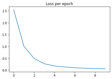
[epoch: 1], loss: 2.5530346045055703
[epoch: 2], loss: 1.0115441271017367
[epoch: 3], loss: 0.4945105895776768
[epoch: 4], loss: 0.26980520496116406
[epoch: 5], loss: 0.176137422897979
[epoch: 6], loss: 0.1321992253904276
[epoch: 7], loss: 0.10100276394910408
[epoch: 8], loss: 0.08020458255299875
[epoch: 9], loss: 0.06571114718797659
[epoch: 10], loss: 0.05607737598425833
import matplotlib.pyplot as plt
plt.plot(epoch_loss)
plt.title('Loss per epoch')
plt.show()