고객이탈예측 with Kaggle API, SMOTE
데이터 분석 문제 정의
- 문제 정의 :고객 이탈 여부 예측. 주어진 변수에 대해 이탈할 것인지 아닌지 0, 1로 예측하는 Binary Classification.
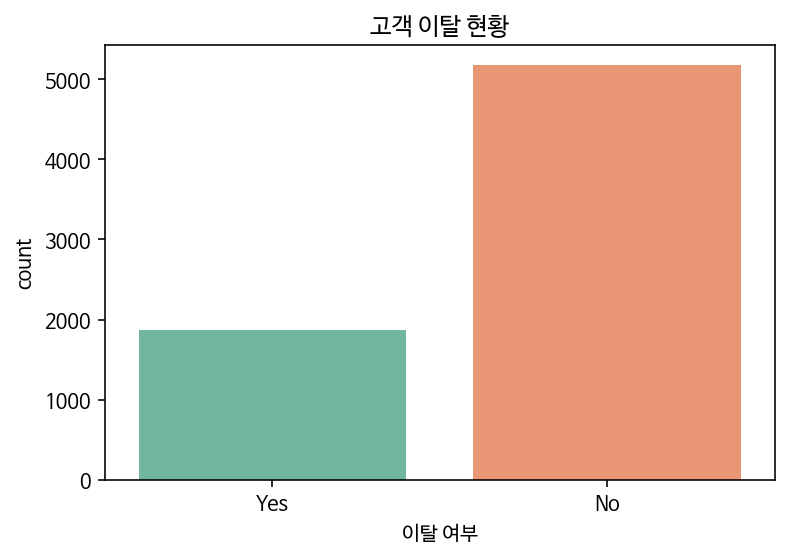
- 대상 데이터 : 캐글 Telco Customer Churn 데이터셋. 고객 이탈인 Yes가 No보다 적은 불균형 데이터이다.
Part1. 데이터 로드 & 데이터 정제
데이터 로드 with Kaggle API
!pip install kaggle
from google.colab import files
files.upload()
Requirement already satisfied: kaggle in /usr/local/lib/python3.7/dist-packages (1.5.12)
Requirement already satisfied: certifi in /usr/local/lib/python3.7/dist-packages (from kaggle) (2020.12.5)
Requirement already satisfied: six>=1.10 in /usr/local/lib/python3.7/dist-packages (from kaggle) (1.15.0)
Requirement already satisfied: urllib3 in /usr/local/lib/python3.7/dist-packages (from kaggle) (1.24.3)
Requirement already satisfied: python-dateutil in /usr/local/lib/python3.7/dist-packages (from kaggle) (2.8.1)
Requirement already satisfied: requests in /usr/local/lib/python3.7/dist-packages (from kaggle) (2.23.0)
Requirement already satisfied: python-slugify in /usr/local/lib/python3.7/dist-packages (from kaggle) (5.0.2)
Requirement already satisfied: tqdm in /usr/local/lib/python3.7/dist-packages (from kaggle) (4.41.1)
Requirement already satisfied: idna<3,>=2.5 in /usr/local/lib/python3.7/dist-packages (from requests->kaggle) (2.10)
Requirement already satisfied: chardet<4,>=3.0.2 in /usr/local/lib/python3.7/dist-packages (from requests->kaggle) (3.0.4)
Requirement already satisfied: text-unidecode>=1.3 in /usr/local/lib/python3.7/dist-packages (from python-slugify->kaggle) (1.3)
!ls -1ha kaggle.json
kaggle.json
!mkdir -p ~/.kaggle
!cp kaggle.json ~/.kaggle/
!chmod 600 ~/.kaggle/kaggle.json
!kaggle datasets download -d blastchar/telco-customer-churn
Downloading telco-customer-churn.zip to /content
  0% 0.00/172k [00:00<?, ?B/s]
100% 172k/172k [00:00<00:00, 52.7MB/s]
!unzip telco-customer-churn.zip
!ls
Archive:  telco-customer-churn.zip
  inflating: WA_Fn-UseC_-Telco-Customer-Churn.csv
kaggle.json  telco-customer-churn.zip
sample_data  WA_Fn-UseC_-Telco-Customer-Churn.csv
## 시각화 라이브러리 로드
import seaborn as sns
import matplotlib.pyplot as plt
%matplotlib inline

# 나눔고딕 설치
!apt -qq -y install fonts-nanum > /dev/null
import matplotlib.font_manager as fm
fontpath = '/usr/share/fonts/truetype/nanum/NanumBarunGothic.ttf'
font = fm.FontProperties(fname=fontpath, size=9)
fm._rebuild()

# 그래프에 retina display 적용
%config InlineBackend.figure_format = 'retina'

# Colab 의 한글 폰트 설정
plt.rc('font', family='NanumBarunGothic')
WARNING: apt does not have a stable CLI interface. Use with caution in scripts.
데이터 상세
- Churn : 고객의 이탈여부 : 목적변수
- gender : 성별
- SeniorCitizen : 연장자 여부
- Partner : 배우자 유무
- Dependents : 부양가족 유무
- tenure : 고객이 회사에 머물렀던 개월 수
- PhoneService : 폰 서비스 받는지 유무
- MultipleLines : 고객이 여러 회선을 사용하는지
- InternetService : 인터넷 서비스 제공 방법
- OnlineSecurity : 고객의 온라인 보안 여부
- OnlineBackup : 고객의 온라인 백업 여부
- DeviceProtection : 고객에게 기기보호 기능이 있는지 여부
- TechSupport : 고객이 기술 지원을 받았는지 여부
- StreamingTV : 고객이 스트리밍 TV를 가지고 있는지 여부
- StreamingMovies : 고객이 영화를 스트리밍 하는지 여부
- Contract : 고객의 계약기간
- PaperlessBilling : 고객의 종이없는 청구서 수신여부
- PaymentMethod : 고객의 결제수단 ( 전자우편, 우편수표, 은행송금(자동), 신용카드(자동) )
- MonthlyCharges : 매월 고객에게 청구되는 금액
- TotalCharges : 고객에게 청구된 총 금액
import pandas as pd

df = pd.read_csv("./WA_Fn-UseC_-Telco-Customer-Churn.csv")
df.head(3)
| customerID | gender | SeniorCitizen | Partner | Dependents | tenure | PhoneService | MultipleLines | InternetService | OnlineSecurity | OnlineBackup | DeviceProtection | TechSupport | StreamingTV | StreamingMovies | Contract | PaperlessBilling | PaymentMethod | MonthlyCharges | TotalCharges | Churn | |
|---|---|---|---|---|---|---|---|---|---|---|---|---|---|---|---|---|---|---|---|---|---|
| 0 | 7590-VHVEG | Female | 0 | Yes | No | 1 | No | No phone service | DSL | No | Yes | No | No | No | No | Month-to-month | Yes | Electronic check | 29.85 | 29.85 | No |
| 1 | 5575-GNVDE | Male | 0 | No | No | 34 | Yes | No | DSL | Yes | No | Yes | No | No | No | One year | No | Mailed check | 56.95 | 1889.5 | No |
| 2 | 3668-QPYBK | Male | 0 | No | No | 2 | Yes | No | DSL | Yes | Yes | No | No | No | No | Month-to-month | Yes | Mailed check | 53.85 | 108.15 | Yes |
## head, describe, shape, info
display(df.head(3))
display(df.describe())
display(df.shape)
display(df.info())
| customerID | gender | SeniorCitizen | Partner | Dependents | tenure | PhoneService | MultipleLines | InternetService | OnlineSecurity | OnlineBackup | DeviceProtection | TechSupport | StreamingTV | StreamingMovies | Contract | PaperlessBilling | PaymentMethod | MonthlyCharges | TotalCharges | Churn | |
|---|---|---|---|---|---|---|---|---|---|---|---|---|---|---|---|---|---|---|---|---|---|
| 0 | 7590-VHVEG | Female | 0 | Yes | No | 1 | No | No phone service | DSL | No | Yes | No | No | No | No | Month-to-month | Yes | Electronic check | 29.85 | 29.85 | No |
| 1 | 5575-GNVDE | Male | 0 | No | No | 34 | Yes | No | DSL | Yes | No | Yes | No | No | No | One year | No | Mailed check | 56.95 | 1889.5 | No |
| 2 | 3668-QPYBK | Male | 0 | No | No | 2 | Yes | No | DSL | Yes | Yes | No | No | No | No | Month-to-month | Yes | Mailed check | 53.85 | 108.15 | Yes |
| SeniorCitizen | tenure | MonthlyCharges | |
|---|---|---|---|
| count | 7043.000000 | 7043.000000 | 7043.000000 |
| mean | 0.162147 | 32.371149 | 64.761692 |
| std | 0.368612 | 24.559481 | 30.090047 |
| min | 0.000000 | 0.000000 | 18.250000 |
| 25% | 0.000000 | 9.000000 | 35.500000 |
| 50% | 0.000000 | 29.000000 | 70.350000 |
| 75% | 0.000000 | 55.000000 | 89.850000 |
| max | 1.000000 | 72.000000 | 118.750000 |
(7043, 21)


<class 'pandas.core.frame.DataFrame'>
RangeIndex: 7043 entries, 0 to 7042
Data columns (total 21 columns):
 #   Column            Non-Null Count  Dtype
---  ------            --------------  -----
 0   customerID        7043 non-null   object
 1   gender            7043 non-null   object
 2   SeniorCitizen     7043 non-null   int64
 3   Partner           7043 non-null   object
 4   Dependents        7043 non-null   object
 5   tenure            7043 non-null   int64
 6   PhoneService      7043 non-null   object
 7   MultipleLines     7043 non-null   object
 8   InternetService   7043 non-null   object
 9   OnlineSecurity    7043 non-null   object
 10  OnlineBackup      7043 non-null   object
 11  DeviceProtection  7043 non-null   object
 12  TechSupport       7043 non-null   object
 13  StreamingTV       7043 non-null   object
 14  StreamingMovies   7043 non-null   object
 15  Contract          7043 non-null   object
 16  PaperlessBilling  7043 non-null   object
 17  PaymentMethod     7043 non-null   object
 18  MonthlyCharges    7043 non-null   float64
 19  TotalCharges      7043 non-null   object
 20  Churn             7043 non-null   object
dtypes: float64(1), int64(2), object(18)
memory usage: 1.1+ MB


None
# 불균형 데이터인지 확인하기
import warnings
warnings.filterwarnings(action='ignore')

ax = sns.countplot(data = df, x='Churn', palette="Set2", order = ["Yes", "No"])
ax.set_title('고객 이탈 현황')
ax.set_xlabel('이탈 여부')
plt.show()
데이터 정제 - 1) customerid 삭제
- ‘customerid’ 컬럼은 이탈 예측에 있어 중요한 정보를 제공하지 않으므로 삭제한다.
df.drop(labels=['customerID'], axis=1, inplace=True)
df.head(2)
| gender | SeniorCitizen | Partner | Dependents | tenure | PhoneService | MultipleLines | InternetService | OnlineSecurity | OnlineBackup | DeviceProtection | TechSupport | StreamingTV | StreamingMovies | Contract | PaperlessBilling | PaymentMethod | MonthlyCharges | TotalCharges | Churn | |
|---|---|---|---|---|---|---|---|---|---|---|---|---|---|---|---|---|---|---|---|---|
| 0 | Female | 0 | Yes | No | 1 | No | No phone service | DSL | No | Yes | No | No | No | No | Month-to-month | Yes | Electronic check | 29.85 | 29.85 | No |
| 1 | Male | 0 | No | No | 34 | Yes | No | DSL | Yes | No | Yes | No | No | No | One year | No | Mailed check | 56.95 | 1889.5 | No |
데이터 정제 - 2) Null처리
## 컬럼명 rename
value_mapper = {'Female': 'F', 'Male': 'M', 'Yes': 'Y', 'No': 'N',
                'No phone service': 'No phone', 'Fiber optic': 'Fiber',
                'No internet service': 'No internet', 'Month-to-month': 'Monthly',
                'Bank transfer (automatic)': 'Bank transfer',
                'Credit card (automatic)': 'Credit card',
                'One year': '1 yr', 'Two year': '2 yr'}
df.replace(to_replace=value_mapper, inplace=True)
df.columns = [label.lower() for label in df.columns]
df.head(10).T
| 0 | 1 | 2 | 3 | 4 | 5 | 6 | 7 | 8 | 9 | |
|---|---|---|---|---|---|---|---|---|---|---|
| gender | F | M | M | M | F | F | M | F | F | M |
| seniorcitizen | 0 | 0 | 0 | 0 | 0 | 0 | 0 | 0 | 0 | 0 |
| partner | Y | N | N | N | N | N | N | N | Y | N |
| dependents | N | N | N | N | N | N | Y | N | N | Y |
| tenure | 1 | 34 | 2 | 45 | 2 | 8 | 22 | 10 | 28 | 62 |
| phoneservice | N | Y | Y | N | Y | Y | Y | N | Y | Y |
| multiplelines | No phone | N | N | No phone | N | Y | Y | No phone | Y | N |
| internetservice | DSL | DSL | DSL | DSL | Fiber | Fiber | Fiber | DSL | Fiber | DSL |
| onlinesecurity | N | Y | Y | Y | N | N | N | Y | N | Y |
| onlinebackup | Y | N | Y | N | N | N | Y | N | N | Y |
| deviceprotection | N | Y | N | Y | N | Y | N | N | Y | N |
| techsupport | N | N | N | Y | N | N | N | N | Y | N |
| streamingtv | N | N | N | N | N | Y | Y | N | Y | N |
| streamingmovies | N | N | N | N | N | Y | N | N | Y | N |
| contract | Monthly | 1 yr | Monthly | 1 yr | Monthly | Monthly | Monthly | Monthly | Monthly | 1 yr |
| paperlessbilling | Y | N | Y | N | Y | Y | Y | N | Y | N |
| paymentmethod | Electronic check | Mailed check | Mailed check | Bank transfer | Electronic check | Electronic check | Credit card | Mailed check | Electronic check | Bank transfer |
| monthlycharges | 29.85 | 56.95 | 53.85 | 42.3 | 70.7 | 99.65 | 89.1 | 29.75 | 104.8 | 56.15 |
| totalcharges | 29.85 | 1889.5 | 108.15 | 1840.75 | 151.65 | 820.5 | 1949.4 | 301.9 | 3046.05 | 3487.95 |
| churn | N | N | Y | N | Y | Y | N | N | Y | N |
## 형변환 : TotalCharges 컬럼 object -> float로 형변환
df['totalcharges'] = pd.to_numeric(df['totalcharges'], errors='coerce')
df['totalcharges'].head()
0      29.85
1    1889.50
2     108.15
3    1840.75
4     151.65
Name: totalcharges, dtype: float64
## 결측치 확인
df.isnull().sum()
gender               0
seniorcitizen        0
partner              0
dependents           0
tenure               0
phoneservice         0
multiplelines        0
internetservice      0
onlinesecurity       0
onlinebackup         0
deviceprotection     0
techsupport          0
streamingtv          0
streamingmovies      0
contract             0
paperlessbilling     0
paymentmethod        0
monthlycharges       0
totalcharges        11
churn                0
dtype: int64
## Null값 확인
import numpy as np

df[np.isnan(df['totalcharges'])]
| gender | seniorcitizen | partner | dependents | tenure | phoneservice | multiplelines | internetservice | onlinesecurity | onlinebackup | deviceprotection | techsupport | streamingtv | streamingmovies | contract | paperlessbilling | paymentmethod | monthlycharges | totalcharges | churn | |
|---|---|---|---|---|---|---|---|---|---|---|---|---|---|---|---|---|---|---|---|---|
| 488 | F | 0 | Y | Y | 0 | N | No phone | DSL | Y | N | Y | Y | Y | N | 2 yr | Y | Bank transfer | 52.55 | NaN | N |
| 753 | M | 0 | N | Y | 0 | Y | N | N | No internet | No internet | No internet | No internet | No internet | No internet | 2 yr | N | Mailed check | 20.25 | NaN | N |
| 936 | F | 0 | Y | Y | 0 | Y | N | DSL | Y | Y | Y | N | Y | Y | 2 yr | N | Mailed check | 80.85 | NaN | N |
| 1082 | M | 0 | Y | Y | 0 | Y | Y | N | No internet | No internet | No internet | No internet | No internet | No internet | 2 yr | N | Mailed check | 25.75 | NaN | N |
| 1340 | F | 0 | Y | Y | 0 | N | No phone | DSL | Y | Y | Y | Y | Y | N | 2 yr | N | Credit card | 56.05 | NaN | N |
| 3331 | M | 0 | Y | Y | 0 | Y | N | N | No internet | No internet | No internet | No internet | No internet | No internet | 2 yr | N | Mailed check | 19.85 | NaN | N |
| 3826 | M | 0 | Y | Y | 0 | Y | Y | N | No internet | No internet | No internet | No internet | No internet | No internet | 2 yr | N | Mailed check | 25.35 | NaN | N |
| 4380 | F | 0 | Y | Y | 0 | Y | N | N | No internet | No internet | No internet | No internet | No internet | No internet | 2 yr | N | Mailed check | 20.00 | NaN | N |
| 5218 | M | 0 | Y | Y | 0 | Y | N | N | No internet | No internet | No internet | No internet | No internet | No internet | 1 yr | Y | Mailed check | 19.70 | NaN | N |
| 6670 | F | 0 | Y | Y | 0 | Y | Y | DSL | N | Y | Y | Y | Y | N | 2 yr | N | Mailed check | 73.35 | NaN | N |
| 6754 | M | 0 | N | Y | 0 | Y | Y | DSL | Y | Y | N | Y | N | N | 2 yr | Y | Bank transfer | 61.90 | NaN | N |
df[df['tenure'] == 0].index # totalcharges(지불금액)도 비어있고, tenure(유지개월수)도 0이다.
Int64Index([488, 753, 936, 1082, 1340, 3331, 3826, 4380, 5218, 6670, 6754], dtype='int64')
# 따라서 tenure가 0인 행을 삭제한다
df.drop(labels=df[df['tenure'] == 0].index, axis=0, inplace=True)
df[df['tenure'] == 0].index
Int64Index([], dtype='int64')
df.isnull().sum()
gender              0
seniorcitizen       0
partner             0
dependents          0
tenure              0
phoneservice        0
multiplelines       0
internetservice     0
onlinesecurity      0
onlinebackup        0
deviceprotection    0
techsupport         0
streamingtv         0
streamingmovies     0
contract            0
paperlessbilling    0
paymentmethod       0
monthlycharges      0
totalcharges        0
churn               0
dtype: int64
데이터 정제 - 3) 카테고리형 변수 형변환
def summarize_categoricals(df, show_levels=False):
    data = [[df[c].unique(), len(df[c].unique()), df[c].isnull().sum()] for c in df.columns]
    df_temp = pd.DataFrame(data, index=df.columns,
                           columns=['Levels', 'No. of Levels', 'No. of Missing Values'])
    return df_temp.iloc[:, 0 if show_levels else 1:]


def find_categorical(df, cutoff=10):
    cat_cols = []
    for col in df.columns:
        if len(df[col].unique()) <= cutoff:
            cat_cols.append(col)
    return cat_cols


def to_categorical(columns, df):
    for col in columns:
        df[col] = df[col].astype('category')
    return df
summarize_categoricals(df, show_levels=True)
| Levels | No. of Levels | No. of Missing Values | |
|---|---|---|---|
| gender | [F, M] | 2 | 0 |
| seniorcitizen | [0, 1] | 2 | 0 |
| partner | [Y, N] | 2 | 0 |
| dependents | [N, Y] | 2 | 0 |
| tenure | [1, 34, 2, 45, 8, 22, 10, 28, 62, 13, 16, 58, ... | 72 | 0 |
| phoneservice | [N, Y] | 2 | 0 |
| multiplelines | [No phone, N, Y] | 3 | 0 |
| internetservice | [DSL, Fiber, N] | 3 | 0 |
| onlinesecurity | [N, Y, No internet] | 3 | 0 |
| onlinebackup | [Y, N, No internet] | 3 | 0 |
| deviceprotection | [N, Y, No internet] | 3 | 0 |
| techsupport | [N, Y, No internet] | 3 | 0 |
| streamingtv | [N, Y, No internet] | 3 | 0 |
| streamingmovies | [N, Y, No internet] | 3 | 0 |
| contract | [Monthly, 1 yr, 2 yr] | 3 | 0 |
| paperlessbilling | [Y, N] | 2 | 0 |
| paymentmethod | [Electronic check, Mailed check, Bank transfer... | 4 | 0 |
| monthlycharges | [29.85, 56.95, 53.85, 42.3, 70.7, 99.65, 89.1,... | 1584 | 0 |
| totalcharges | [29.85, 1889.5, 108.15, 1840.75, 151.65, 820.5... | 6530 | 0 |
| churn | [N, Y] | 2 | 0 |
df = to_categorical(find_categorical(df), df)
df.info()
<class 'pandas.core.frame.DataFrame'>
Int64Index: 7032 entries, 0 to 7042
Data columns (total 20 columns):
 #   Column            Non-Null Count  Dtype
---  ------            --------------  -----
 0   gender            7032 non-null   category
 1   seniorcitizen     7032 non-null   category
 2   partner           7032 non-null   category
 3   dependents        7032 non-null   category
 4   tenure            7032 non-null   int64
 5   phoneservice      7032 non-null   category
 6   multiplelines     7032 non-null   category
 7   internetservice   7032 non-null   category
 8   onlinesecurity    7032 non-null   category
 9   onlinebackup      7032 non-null   category
 10  deviceprotection  7032 non-null   category
 11  techsupport       7032 non-null   category
 12  streamingtv       7032 non-null   category
 13  streamingmovies   7032 non-null   category
 14  contract          7032 non-null   category
 15  paperlessbilling  7032 non-null   category
 16  paymentmethod     7032 non-null   category
 17  monthlycharges    7032 non-null   float64
 18  totalcharges      7032 non-null   float64
 19  churn             7032 non-null   category
dtypes: category(17), float64(2), int64(1)
memory usage: 338.2 KB
new_order = list(df.columns)
new_order.insert(16, new_order.pop(4))
df = df[new_order]
df.head(2)
| gender | seniorcitizen | partner | dependents | phoneservice | multiplelines | internetservice | onlinesecurity | onlinebackup | deviceprotection | techsupport | streamingtv | streamingmovies | contract | paperlessbilling | paymentmethod | tenure | monthlycharges | totalcharges | churn | |
|---|---|---|---|---|---|---|---|---|---|---|---|---|---|---|---|---|---|---|---|---|
| 0 | F | 0 | Y | N | N | No phone | DSL | N | Y | N | N | N | N | Monthly | Y | Electronic check | 1 | 29.85 | 29.85 | N |
| 1 | M | 0 | N | N | Y | N | DSL | Y | N | Y | N | N | N | 1 yr | N | Mailed check | 34 | 56.95 | 1889.50 | N |
Part2. 데이터 전처리
correlation 분석 - 1) 연속형 변수간 correlation 분석
sns.heatmap(data=df[['tenure', 'monthlycharges', 'totalcharges']].corr(),
            annot=True, cmap='coolwarm');
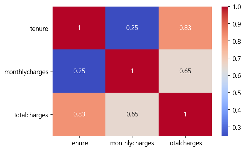
위에서 알 수 있듯, ‘totalcharge(총요금)’은 고객이 머무르던 동안의 총 월요금을 합한 것이므로 ‘monthlycharges(월요금)’과 ‘tenure(고객이 머무른 기간)’과 높은 상관관계가 있다.
correlation 분석 - 2) 범주형 변수간 correlation 분석
- 변수들의 연속성 여부와 관계없이 correlation을 분석하고 싶고, 측정치 분포 표준화가 되어있지 않으므로, Cramer V 계수를 사용한다.
- V 계수는 서로 최대의 관련성을 가질때 1, 아무 상관이 없을때 0으로 표현된다.
# Cramer V 계수 계산
from scipy.stats import chi2_contingency

def cramers_corrected_stat(contingency_table):
    chi2 = chi2_contingency(contingency_table)[0]
    n = contingency_table.sum().sum()
    phi2 = chi2/n

    r, k = contingency_table.shape
    r_corrected = r - (((r-1)**2)/(n-1))
    k_corrected = k - (((k-1)**2)/(n-1))
    phi2_corrected = max(0, phi2 - ((k-1)*(r-1))/(n-1))

    return (phi2_corrected / min( (k_corrected-1), (r_corrected-1)))**0.5
# 범주형 변수간 Cramer V 계수 계산
def categorical_corr_matrix(df):
    df = df.select_dtypes(include='category')
    cols = df.columns
    n = len(cols)
    corr_matrix = pd.DataFrame(np.zeros(shape=(n, n)), index=cols, columns=cols)

    for col1 in cols:
        for col2 in cols:
            if col1 == col2:
                corr_matrix.loc[col1, col2] = 1
                break
            df_crosstab = pd.crosstab(df[col1], df[col2], dropna=False)
            corr_matrix.loc[col1, col2] = cramers_corrected_stat(df_crosstab)

    corr_matrix += np.tril(corr_matrix, k=-1).T
    return corr_matrix
fig, ax = plt.subplots(figsize=(15, 10))
sns.heatmap(categorical_corr_matrix(df), annot=True, cmap='coolwarm',
            cbar_kws={'aspect': 50}, square=True, ax=ax)
plt.xticks(rotation=60);
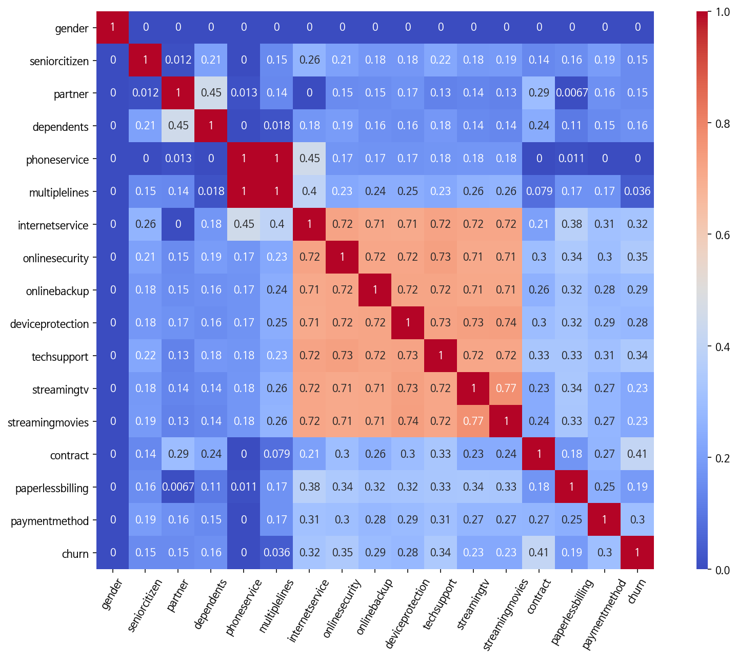
- 전화 서비스가 없는 사람들은 여러 회선을 가질 수 없기 때문에 ‘phone service(전화 서비스)’와 ‘multiple lines(다중 회선)’간에는 약간의 상관 관계가 있다. 따라서 특정 고객이 전화 서비스에 가입되어 있지 않다는 것을 알면 고객이 여러 회선을 가지고 있지 않다고 알 수 있다. 마찬가지로 ‘internet service’와 ‘online security’, ‘online backup’, ‘device protection’, ‘streaming tv’, ‘streaming movies’간에도 상관 관계가 있다.
- 만약 계산량을 줄이기 위해 feature를 줄인다면 고려해볼만한 항목이다.
- 또한 상관관계가 높은 것들을 위주로 원-핫 인코딩을 해볼 수도 있겠다.
Train-Test split
- 테스트 데이터 세트를 Stratified 방식으로 추출해 훈련 데이터 세트와 테스트 데이터 세트의 레이블 분포도를 서로 동일하게 만든다.
x = df.iloc[:, :-1]
y = df['churn']

categorical_columns = list(x.select_dtypes(include='category').columns)
numeric_columns = list(x.select_dtypes(exclude='category').columns)
from sklearn.model_selection import train_test_split

data_splits = train_test_split(x, y, test_size=0.25, random_state=0,
                               shuffle=True, stratify=y)
x_train, x_test, y_train, y_test = data_splits

print('Train 데이터 레이블 값 비율')
print(y_train.value_counts()/y_train.shape[0]*100)
print('Test 데이터 레이블 값 비율')
print(y_test.value_counts()/y_test.shape[0]*100)
Train 데이터 레이블 값 비율
N    73.416761
Y    26.583239
Name: churn, dtype: float64
Test 데이터 레이블 값 비율
N    73.435722
Y    26.564278
Name: churn, dtype: float64
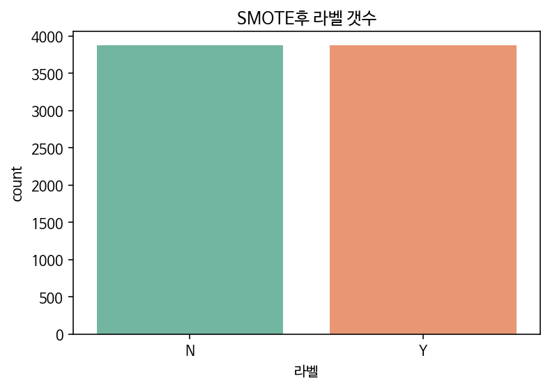
**불균형 데이터 처리 : SMOTENC를 이용한 OverSampling
- 라벨 Y가 N보다 훨씬 적은 불균형데이터이므로 훈련 데이터 셋을 SMOTE로 Over Sampling한다.
- 현재 변수가 연속형 변수와 범주형 변수가 함께 있으므로, SMOTENC를 이용한다.
- 테스트 데이터셋은 건드리지 않아야하므로, split 이후 진행한다.
from imblearn.over_sampling import SMOTENC

smote = SMOTENC(categorical_features=(x_train.dtypes == "category").values,
                random_state=42)

x_train, y_train = smote.fit_resample(x_train, y_train)
pd.Series(y_train).value_counts()
N    3872
Y    3872
dtype: int64
ax = sns.countplot(x=y_train, palette="Set2")
ax.set_title('SMOTE후 라벨 갯수')
ax.set_xlabel('라벨')
plt.show()
Standardization
- 모델 적용 전, 연속형 변수를 표준화한다.
- 피쳐를 표준화하지 않으면, 큰 분산을 갖고 있는 피쳐가 모델 학습에 있어 영향을 더 많이 행사하게 되고, 모델이 다른 피쳐를 학습할 수 없기 때문이다.
- 따라서 연속형 변수를 스케일링한다.
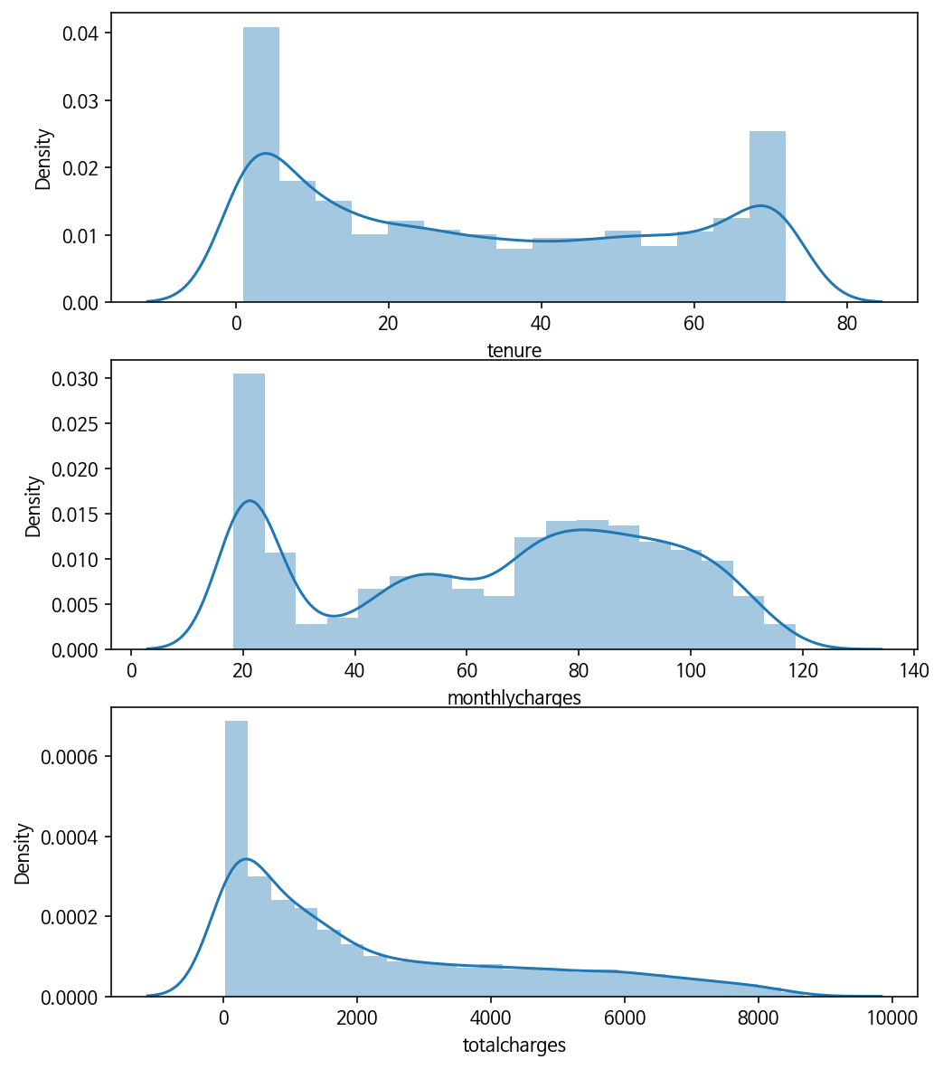
## 기존의 데이터 분포
plt.figure(figsize=(8,10))

plt.subplot(3, 1, 1);
sns.distplot(df['tenure'])

plt.subplot(3, 1, 2);
sns.distplot(df['monthlycharges'])

plt.subplot(3, 1, 3);
sns.distplot(df['totalcharges'])

# Show the plot
plt.show()
데이터 인코딩 : One-hot encoding
- 범주형 변수는 원-핫 인코딩을 통해 숫자형으로 변환한다.
from sklearn.compose import ColumnTransformer
from sklearn.preprocessing import OneHotEncoder, StandardScaler, LabelEncoder

categorical_columns = list(x.select_dtypes(include='category').columns)
numeric_columns = list(x.select_dtypes(exclude='category').columns)

## Column Transformer
transformers = [('one_hot_encoder',
                  OneHotEncoder(drop='first',dtype='int'),
                  categorical_columns),
                ('standard_scaler', StandardScaler(), numeric_columns)]
x_trans = ColumnTransformer(transformers, remainder='passthrough')

## Applying Column Transformer
x_train = x_trans.fit_transform(pd.DataFrame(x_train, columns=categorical_columns+numeric_columns))
x_test = x_trans.transform(pd.DataFrame(x_test))

## Label encoding
y_trans = LabelEncoder()
y_train = y_trans.fit_transform(pd.DataFrame(y_train))
y_test = y_trans.transform(pd.DataFrame(y_test))


## Save feature names after one-hot encoding for feature importances plots
feature_names = list(x_trans.named_transformers_['one_hot_encoder'] \
                            .get_feature_names(input_features=categorical_columns))
feature_names = feature_names + numeric_columns
# SMOTE 전후 비교를 위한 data set
x_train_o, x_test_o, y_train_o, y_test_o = data_splits

x_train_o = x_trans.fit_transform(pd.DataFrame(x_train_o, columns=categorical_columns+numeric_columns))
x_test_o = x_trans.transform(pd.DataFrame(x_test_o))

y_train_o = y_trans.fit_transform(pd.DataFrame(y_train_o))
y_test_o = y_trans.transform(pd.DataFrame(y_test_o))
# 비교를 위한 데이터프레임화
after_prep = pd.DataFrame(x_train, columns=feature_names)
after_prep.head(3)
| gender_M | seniorcitizen_1 | partner_Y | dependents_Y | phoneservice_Y | multiplelines_No phone | multiplelines_Y | internetservice_Fiber | internetservice_N | onlinesecurity_No internet | onlinesecurity_Y | onlinebackup_No internet | onlinebackup_Y | deviceprotection_No internet | deviceprotection_Y | techsupport_No internet | techsupport_Y | streamingtv_No internet | streamingtv_Y | streamingmovies_No internet | streamingmovies_Y | contract_2 yr | contract_Monthly | paperlessbilling_Y | paymentmethod_Credit card | paymentmethod_Electronic check | paymentmethod_Mailed check | tenure | monthlycharges | totalcharges | |
|---|---|---|---|---|---|---|---|---|---|---|---|---|---|---|---|---|---|---|---|---|---|---|---|---|---|---|---|---|---|---|
| 0 | 0.0 | 1.0 | 0.0 | 0.0 | 1.0 | 0.0 | 0.0 | 1.0 | 0.0 | 0.0 | 0.0 | 0.0 | 1.0 | 0.0 | 0.0 | 0.0 | 0.0 | 0.0 | 1.0 | 0.0 | 0.0 | 0.0 | 1.0 | 1.0 | 0.0 | 0.0 | 0.0 | -1.071261 | 0.554873 | -0.861789 |
| 1 | 0.0 | 0.0 | 1.0 | 0.0 | 1.0 | 0.0 | 0.0 | 0.0 | 1.0 | 1.0 | 0.0 | 1.0 | 0.0 | 1.0 | 0.0 | 1.0 | 0.0 | 1.0 | 0.0 | 1.0 | 0.0 | 0.0 | 0.0 | 0.0 | 0.0 | 0.0 | 0.0 | 0.900700 | -1.668186 | -0.521394 |
| 2 | 1.0 | 0.0 | 0.0 | 0.0 | 1.0 | 0.0 | 0.0 | 0.0 | 1.0 | 1.0 | 0.0 | 1.0 | 0.0 | 1.0 | 0.0 | 1.0 | 0.0 | 1.0 | 0.0 | 1.0 | 0.0 | 0.0 | 1.0 | 1.0 | 0.0 | 1.0 | 0.0 | -0.609738 | -1.669941 | -0.821179 |
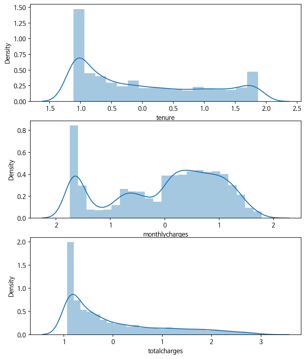
## 표준화 이후 데이터 분포
import warnings
warnings.filterwarnings(action='ignore')

plt.figure(figsize=(8,10))

plt.subplot(3, 1, 1);
sns.distplot(after_prep['tenure'])

plt.subplot(3, 1, 2);
sns.distplot(after_prep['monthlycharges'])

plt.subplot(3, 1, 3);
sns.distplot(after_prep['totalcharges'])

# Show the plot
plt.show()
## 원핫 인코딩 이후 범주형 변수 상태
after_prep.iloc[:3,:-3]
| gender_M | seniorcitizen_1 | partner_Y | dependents_Y | phoneservice_Y | multiplelines_No phone | multiplelines_Y | internetservice_Fiber | internetservice_N | onlinesecurity_No internet | onlinesecurity_Y | onlinebackup_No internet | onlinebackup_Y | deviceprotection_No internet | deviceprotection_Y | techsupport_No internet | techsupport_Y | streamingtv_No internet | streamingtv_Y | streamingmovies_No internet | streamingmovies_Y | contract_2 yr | contract_Monthly | paperlessbilling_Y | paymentmethod_Credit card | paymentmethod_Electronic check | paymentmethod_Mailed check | |
|---|---|---|---|---|---|---|---|---|---|---|---|---|---|---|---|---|---|---|---|---|---|---|---|---|---|---|---|
| 0 | 0.0 | 1.0 | 0.0 | 0.0 | 1.0 | 0.0 | 0.0 | 1.0 | 0.0 | 0.0 | 0.0 | 0.0 | 1.0 | 0.0 | 0.0 | 0.0 | 0.0 | 0.0 | 1.0 | 0.0 | 0.0 | 0.0 | 1.0 | 1.0 | 0.0 | 0.0 | 0.0 |
| 1 | 0.0 | 0.0 | 1.0 | 0.0 | 1.0 | 0.0 | 0.0 | 0.0 | 1.0 | 1.0 | 0.0 | 1.0 | 0.0 | 1.0 | 0.0 | 1.0 | 0.0 | 1.0 | 0.0 | 1.0 | 0.0 | 0.0 | 0.0 | 0.0 | 0.0 | 0.0 | 0.0 |
| 2 | 1.0 | 0.0 | 0.0 | 0.0 | 1.0 | 0.0 | 0.0 | 0.0 | 1.0 | 1.0 | 0.0 | 1.0 | 0.0 | 1.0 | 0.0 | 1.0 | 0.0 | 1.0 | 0.0 | 1.0 | 0.0 | 0.0 | 1.0 | 1.0 | 0.0 | 1.0 | 0.0 |
Part3. 데이터 모델링
- 모델 학습/예측 : Logistic Regression(+Cross Validation), Random Forest, AdaBoost, XGBoost, KNN
- 학습 데이터 셋이 작기 때문에 Cross Validation을 사용한다.
- 성능평가 : Confusion Matrix, Accuracy, precision, recall, F1-score, AUC -> 이상탐지이므로 주로 F1 Score와 AUC를 중심으로 본다.
- 특히, SMOTE를 적용하면 재현율(recall)은 높아지나, 정밀도(precision)는 낮아지는 것이 일반적이다. 따라서 SMOTE 적용의 효과를 보기 위해서는 SMOTE 전후의 재현율 증가율과, 정밀도 감소율을 살펴보려고 한다.
# 모델 평가 함수 정의
from sklearn.metrics import accuracy_score, precision_score , recall_score , confusion_matrix, roc_auc_score, f1_score
from sklearn.metrics import plot_confusion_matrix

def get_clf_eval(y_test , pred):
    confusion = confusion_matrix( y_test, pred)
    accuracy = accuracy_score(y_test , pred)
    precision = precision_score(y_test , pred)
    recall = recall_score(y_test , pred)
    f1 = f1_score(y_test,pred)
    # ROC-AUC 추가
    roc_auc = roc_auc_score(y_test, pred)
    print('오차 행렬')
    print(confusion)
    # ROC-AUC print 추가
    print('정확도: {0:.4f}, 정밀도: {1:.4f}, 재현율: {2:.4f}, F1: {3:.4f}, AUC:{4:.4f}'.format(accuracy, precision, recall, f1, roc_auc))
# 모델 학습/예측 함수 정의
def get_model_train_eval(model, ftr_train=None, ftr_test=None, tgt_train=None, tgt_test=None):
    model.fit(ftr_train, tgt_train)
    pred = model.predict(ftr_test)
    pred_proba = model.predict_proba(ftr_test)[:, 1]
    get_clf_eval(tgt_test, pred)
Logistic Regression
## 불균형 데이터 처리(SMOTE) 전 모델 성능
from sklearn.linear_model import LogisticRegressionCV

logit_cv = LogisticRegressionCV(Cs=10, class_weight='balanced', cv=5, dual=False,
                                fit_intercept=True, intercept_scaling=1.0, l1_ratios=None,
                                max_iter=500, multi_class='auto', n_jobs=None,
                                penalty='l1', random_state=0, refit=True,
                                scoring='f1', solver='liblinear', tol=0.0001,
                                verbose=0)

get_model_train_eval(logit_cv, ftr_train=x_train_o, ftr_test=x_test_o, tgt_train=y_train_o, tgt_test=y_test_o)
오차 행렬
[[955 336]
 [100 367]]
정확도: 0.7520, 정밀도: 0.5220, 재현율: 0.7859, F1: 0.6274, AUC:0.7628
## 불균형 데이터 처리(SMOTE) 후 모델 성능
get_model_train_eval(logit_cv, ftr_train=x_train, ftr_test=x_test, tgt_train=y_train, tgt_test=y_test)
오차 행렬
[[993 298]
 [131 336]]
정확도: 0.7560, 정밀도: 0.5300, 재현율: 0.7195, F1: 0.6104, AUC:0.7443
Logistic Regression의 경우, 정밀도는 높아졌지만, SMOTE이후 재현율이 낮아졌다. 왜 그런지 보기 위해 분류 결정 임계값에 따른 정밀도-재현율 곡선을 그려본다.
from sklearn.metrics import precision_recall_curve

def precision_recall_curve_plot(y_test , pred_proba_c1):
    # threshold ndarray와 이 threshold에 따른 정밀도, 재현율 ndarray 추출.
    precisions, recalls, thresholds = precision_recall_curve( y_test, pred_proba_c1)

    # X축을 threshold값으로, Y축은 정밀도, 재현율 값으로 각각 Plot 수행. 정밀도는 점선으로 표시
    plt.figure(figsize=(8,6))
    threshold_boundary = thresholds.shape[0]
    plt.plot(thresholds, precisions[0:threshold_boundary], linestyle='--', label='precision')
    plt.plot(thresholds, recalls[0:threshold_boundary],label='recall')

    # threshold 값 X 축의 Scale을 0.1 단위로 변경
    start, end = plt.xlim()
    plt.xticks(np.round(np.arange(start, end, 0.1),2))

    # x축, y축 label과 legend, 그리고 grid 설정
    plt.xlabel('Threshold value'); plt.ylabel('Precision and Recall value')
    plt.legend(); plt.grid()
    plt.show()

precision_recall_curve_plot(y_test, logit_cv.predict_proba(x_test)[:, 1] )
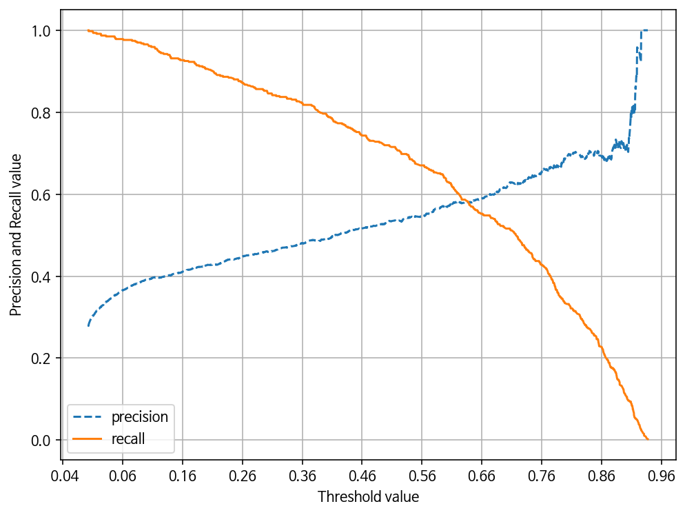
임계값(threshold)을 조정해서 다시 해본다. threshold=0.66
def get_logit_train_eval(model, ftr_train=None, ftr_test=None, tgt_train=None, tgt_test=None):
    model.fit(ftr_train, tgt_train)
    THRESHOLD = 0.66
    pred = np.where(model.predict_proba(ftr_test)[:,1] > THRESHOLD, 1, 0)
    get_clf_eval(tgt_test, pred)
print("### SMOTE전 ###")
get_logit_train_eval(logit_cv, ftr_train=x_train_o, ftr_test=x_test_o, tgt_train=y_train_o, tgt_test=y_test_o)
print("### SMOTE후 ###")
get_logit_train_eval(logit_cv, ftr_train=x_train, ftr_test=x_test, tgt_train=y_train, tgt_test=y_test)
### SMOTE전 ###
오차 행렬
[[1090  201]
 [ 179  288]]
정확도: 0.7838, 정밀도: 0.5890, 재현율: 0.6167, F1: 0.6025, AUC:0.7305
### SMOTE후 ###
오차 행렬
[[1111  180]
 [ 209  258]]
정확도: 0.7787, 정밀도: 0.5890, 재현율: 0.5525, F1: 0.5702, AUC:0.7065
- 임계값을 조정한다고 해도, 임계값 0.90 부근에서 재현율과 정밀도가 극도로 민감해지므로, Logistic Regression 모델의 경우 SMOTE 적용 후 올바른 예측모델이 생성되지 못했다.
- 좋은 SMOTE 모델일수록 재현율 증가율은 높이고 정밀도 감소율은 낮아져야 한다.
Random Forest
from sklearn.ensemble import RandomForestClassifier

random_forest = RandomForestClassifier(class_weight='balanced', criterion='entropy',
                                       max_depth=1, n_estimators=100,
                                       n_jobs=-1, random_state=0)

print("### SMOTE전 ###")
get_model_train_eval(random_forest, ftr_train=x_train_o, ftr_test=x_test_o, tgt_train=y_train_o, tgt_test=y_test_o)
print("### SMOTE후 ###")
get_model_train_eval(random_forest, ftr_train=x_train, ftr_test=x_test, tgt_train=y_train, tgt_test=y_test)
### SMOTE전 ###
오차 행렬
[[850 441]
 [ 86 381]]
정확도: 0.7002, 정밀도: 0.4635, 재현율: 0.8158, F1: 0.5912, AUC:0.7371
### SMOTE후 ###
오차 행렬
[[852 439]
 [ 83 384]]
정확도: 0.7031, 정밀도: 0.4666, 재현율: 0.8223, F1: 0.5953, AUC:0.7411
Random Forest 모델의 경우 SMOTE 적용 후 정밀도와 재현율 모두 증가하여, F1 score와 AUC 또한 증가한 모습을 확인할 수 있다.
AdaBoost
from sklearn.ensemble import AdaBoostClassifier
from sklearn.tree import DecisionTreeClassifier

boosting_dtree = DecisionTreeClassifier(class_weight='balanced',
                                        criterion='entropy',
                                        max_depth=1, random_state=0)
adaboot = AdaBoostClassifier(base_estimator=boosting_dtree,
                             n_estimators=285, learning_rate=0.1,
                             random_state=0)

print("### SMOTE전 ###")
get_model_train_eval(adaboot, ftr_train=x_train_o, ftr_test=x_test_o, tgt_train=y_train_o, tgt_test=y_test_o)
print("### SMOTE후 ###")
get_model_train_eval(adaboot, ftr_train=x_train, ftr_test=x_test, tgt_train=y_train, tgt_test=y_test)
### SMOTE전 ###
오차 행렬
[[933 358]
 [ 89 378]]
정확도: 0.7457, 정밀도: 0.5136, 재현율: 0.8094, F1: 0.6284, AUC:0.7661
### SMOTE후 ###
오차 행렬
[[980 311]
 [117 350]]
정확도: 0.7565, 정밀도: 0.5295, 재현율: 0.7495, F1: 0.6206, AUC:0.7543
AdaBoost의 경우, SMOTE 적용 후 성능이 낮아졌다. 이는, 오분류 시 가중치를 주는 AdaBoost에서는 SMOTE 적용으로 인한 오버샘플링된 데이터가 오히려 혼선을 불러온 것을 의미한다.
XGBoost
from xgboost import XGBClassifier
from sklearn.utils import class_weight

## Compute `class_weights` using sklearn
cls_weight = (y_train.shape[0] - np.sum(y_train)) / np.sum(y_train)

xgb_clf = XGBClassifier(learning_rate=0.01, random_state=0,
                        scale_pos_weight=cls_weight, n_jobs=-1)

print("### SMOTE전 ###")
get_model_train_eval(xgb_clf, ftr_train=x_train_o, ftr_test=x_test_o, tgt_train=y_train_o, tgt_test=y_test_o)
print("### SMOTE후 ###")
get_model_train_eval(xgb_clf, ftr_train=x_train, ftr_test=x_test, tgt_train=y_train, tgt_test=y_test)
### SMOTE전 ###
오차 행렬
[[1197   94]
 [ 271  196]]
정확도: 0.7924, 정밀도: 0.6759, 재현율: 0.4197, F1: 0.5178, AUC:0.6734
### SMOTE후 ###
오차 행렬
[[944 347]
 [119 348]]
정확도: 0.7349, 정밀도: 0.5007, 재현율: 0.7452, F1: 0.5990, AUC:0.7382
XGBoost의 경우 SMOTE 이후 재현율(recall)이 눈에 띄게 높아졌고, 이에 따라 F1 score도 높아졌다.
KNN
from sklearn.neighbors import KNeighborsClassifier

knn = KNeighborsClassifier(n_neighbors=91, p=1,
                           weights='uniform', n_jobs=-1)

print("### SMOTE전 ###")
get_model_train_eval(knn, ftr_train=x_train_o, ftr_test=x_test_o, tgt_train=y_train_o, tgt_test=y_test_o)
print("### SMOTE후 ###")
get_model_train_eval(knn, ftr_train=x_train, ftr_test=x_test, tgt_train=y_train, tgt_test=y_test)
### SMOTE전 ###
오차 행렬
[[1136  155]
 [ 202  265]]
정확도: 0.7969, 정밀도: 0.6310, 재현율: 0.5675, F1: 0.5975, AUC:0.7237
### SMOTE후 ###
오차 행렬
[[834 457]
 [ 70 397]]
정확도: 0.7002, 정밀도: 0.4649, 재현율: 0.8501, F1: 0.6011, AUC:0.7481
KNN의 경우 SMOTE 이후 재현율(recall)이 눈에 띄게 높아졌다.
